I can’t tell based on the re-use of colors, but you may not yet be converged at all given that all of your PMF profiles are different. Error analysis would be helpful. Another method is to generate PMFs for consecutive blocks of time, e.g. 0-2 ns, 2-4 ns, etc. and see if they are changing. As you include fewer frames (by dropping initial frames or calculating a PMF over a shorter time window), the PMF inherently gets noisier due to reduced sampling. The dramatic downward spikes in some of your plots indicate that your profile is pretty sensitive to having adequate sampling in that region of your reaction coordinate.
Dear Dr. Lemkul,
Thank you again for your response. I was trying to learn how to use the error analysis of WHAM. As it was mentioned that users must be very careful not to get underestimated values.
Given that equilibration can happen in the first 1ns of the simulations, I took different time windows and calculated the PMF and the resulting FE. Particularly, I took 1-1.5 ns, 1-2 ns, 1-2.5 ns, 1-3 ns, 1-3.5 ns, … till 1-10 ns of the simulations, and computed the FE. Seems like values sort of converge, despite the PMF not fully covering each other. For instance:

This might be indicative of a convergence in this case. But as you mentioned, I might need to extend some other models to make sure the convergence.
Kind regards,
Ali
Dear Dr. Lemkul,
I computed the standard deviation for all five models and it varries between 1.5 to 2.6 kJ/mol.
I am thinking of extending the simulations for another 5 ns, to make sure/check the convergence.
Can I change the .mdp and use a new .tpr? Doing:
grompp -f new.mdp -c old.tpr -o new.tpr -t old.cpt and then,
mdrun -s new.tpr?
Now if I append to the pull_pullf.xvg and pull_pullx.xvg, shall I use the new.tpr for Umbrella Sampling analysis when all is done?
Thank you for your response in advance.
Kind regards,
Ali
No, what you propose would start the simulation over. You should follow http://manual.gromacs.org/current/user-guide/managing-simulations.html#extending-a-tpr-file
I am not sure if the pullf.xvg and pullx.xvg files can be appended to since they are named differently and do not work in conjunction with -deffnm. You may want to define totally new names for those files in the continuation, then concatenate them after the run completes.
Dear Dr. Lemkul,
Thank you for your kind response.
Great regards,
Ali
Dear Dr. Lemkul,
Finally, after long sampling, the simplest model converged after 23.5 ns. The profile is shown bellow. For the error analysis, I used bootstrapping with -nBootstrap 200 and b-hist method. The std seems to slightly rise with the reaction coordinate and has a mean of around 3.9 kJ/mol.
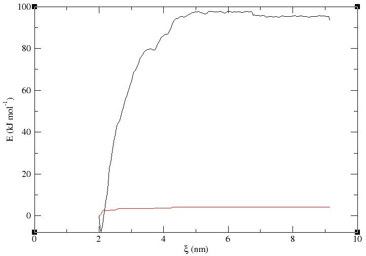
What should be the reported error here for the calculated delta G? is it the error at the minimum of the PMF?
Kind regards,
Ali
The error at the minimum is often reported but if you want to report the ΔG of (un)binding then you would need to compute the difference in free energy between the plateau and the minimum, then propagate the error appropriately, e.g. √(σmin2 + σplateau2).
Dear Dr. Lemkul,
Thank you for your response and kind support.
I would then use the propagation of uncertainties for delta G.
Kind regards,
Ali
Dear Dr. Lemkul,
I am coming back to you on this subject as it does not neem to give me “proper” result.
I am wondering if this is normal not to reach convergence even after very long samplings (88 ns), or have I already!? Here is the example of the free energy change in time (one of the five case studies)
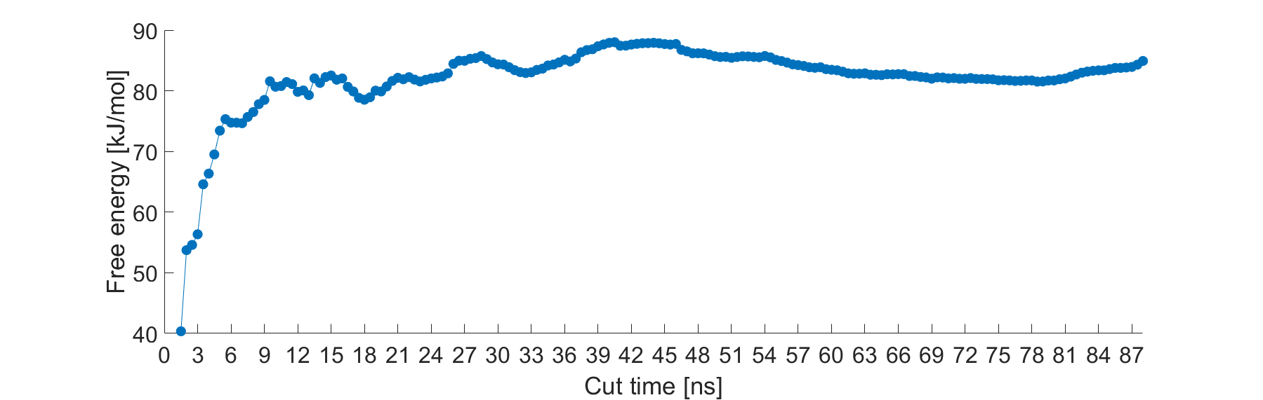
Each point represents calculation of the FE after dropping the first 1 ns of the simulation. However FE does not seem to stabilize…
After performing the error analysis, I have an error of \pm 1.8 kJ/mol at 88 ns of this simulation. I am expecting to get a constant FE after a certain point. But doesn’t seem to happen.
It’s getting a little confusing now. What do you suggest? Any other ways to proceed?
Thank you in advance for your response.
Kind regards,
Ali
Is this the case or is the x-axis correct that it reflects how much time you’re ignoring?
You have an extremely flexible system. It may not be as simple as “remove X ns of simulation time and get a clean result.” Your molecules may be doing different things during different intervals of time. Block averaging results over 10-ns windows (or similar) may be appropriate. The results look fairly stable after about 45 ns. The error analysis produced by gmx wham underestimates the true error, in my experience. So 1.8 kJ/mol is likely a lower limit of the error, meaning you’ve probably been converged for a while.
Dear Dr. Lemkul,
Thank you for your response.
The points refer to calculation of the FE after dropping only the first 1 ns of the simulation, e.g. the point at 44 ns is the FE calculated from 1 ns to 44 ns, and the point at 45 ns is the FE calculated from the 1st ns to the 45th ns of the simulation.
As you also mentioned, the molecule is very flexible, which forms different shapes in different time intervals, but I would certainly do the block averaging to see if I’d get consistent data.
Now for block averaging, shall I have overlap in the blocks? For instance: 1-11, 5-15, 9-19, … or no overlaps such as 1-11, 12-22, 23-33, …?
How much variation in the block averaged results can be expected in a converged simulation?
Thank you again and again.
Kind regards,
Ali
I would use non-overlapping blocks of e.g. 10 ns and see if consecutive blocks are within error of each other. Be careful about clinging to the notion of dropping the first 1 ns; with simulations as long as yours and as flexible as your molecules are, that may not be appropriate. If you just analyze 0-10, 10-20, 20-30, etc. you will be able to see if ΔG is systematically changing or if it has leveled off. You will likely find you need to omit more time than you currently are.
Dear Dr. Lemkul,
Thank you for the clarification. I will proceed with these points.
Kind regards,
Ali